December 31, 2020
Solving Permutation Puzzles Fast with Group Theory and Rust
Published · UpdatedI wrote Cubie and this post back in 2020 and am only now getting around to publishing it in 2026, turns out solving a Rubik's cube is easier than hitting "publish." Cubie is a fast and ergonomic 3x3 Rubik's cube library written in Rust with a group-theory-inspired interface and a solver based on min2phase. The readme covers the full feature set.
Let's see what makes Cubie fast, ergonomic and powerful. Before discussing specifics, let us take a detour, implementing a group theory inspired interface for a simpler puzzle and applying analogous optimizations.
Group Theory
If group theory is something new to you, I recommend 3Blue1Brown's video Group theory and the 196,883-dimensional monster as an engaging introduction. Knowledge of group theory is not required to use the Cubie library or understand this article but is still useful. But before we go further, let me introduce you to our first permutation puzzle to implement.
I have implemented a small permutation puzzle in javascript below, click/touch and drag on tiles to move them about, make sure you understand the mechanics of the puzzle since we are about to implement a library.
The above puzzle, although simpler, is not trivial. If you have trouble solving it, try an easier sub-problem: arrange the tiles such that each row contains tiles of only one colour without regard of the numbers on the tiles.
If you have ever toyed with a Rubik's cube before, the similarities to the above should be obvious.
Our goal is to program a library that represents the states of the game, allows us to perform moves and print the state of the game. We will use a group theoretical representation which I claim is natural and powerful.
Let us Start Programming (I'll explain as we go)
Let's discuss the values at play. The slide puzzle consists of 16 tiles, numbered from 0 through 15, placed on a 4x4 grid. We number the positions on the grid as shown below.
 0  1  2  3    0b00_00 0b00_01 0b00_10 0b00_11
 4  5  6  7    0b01_00 0b01_01 0b01_10 0b01_11
 8  9 10 11    0b10_00 0b10_01 0b10_10 0b10_11
12 13 14 15    0b11_00 0b11_01 0b11_10 0b11_11
Observe that if we define the 0th position to be in the 0th row and 0th column, then the first 2 binary digits (from right to left) specify the column and the second 2 binary digits specify the row for each position number. We will work with the binary representations but for now we just note that the position index is given by
fn position_index(row: u8, col: u8) -> usize {
    debug_assert!(row < 4 && col < 4);
    col | (row << 2) // or equivalently: col + 4*row
}
Then for our array-backed tile map,
#[derive(Copy, Clone, Debug, Eq, PartialEq, Hash)]
pub struct ArrayTileMap{
    map: [u8; 16]
}
We call our state an ArrayTileMap since it maps positions of tiles to their labels; in this way, its behaviour is similar to a HashMap<TilePosition, TileLabel>. However, unlike the hashmap our map has 2 important invariants needed to represent a valid state.
- Every tile position has a tile label, which is statically enforced by having
mapas an array of 16 values one for each position; or mathematically, ArrayTileMap is a well defined function over the domain of tile positions. - There are no duplicated tiles, each position maps to a unique tile label; or mathematically, ArrayTileMap is an injective function. Since we have 16 positions and 16 labels, injectivity implies bijectivity.
Let's make a function to verify these invariants:
impl ArrayTileMap {
    fn is_valid(self) -> bool {
        let mut bitset = 0u16;
        for &label in &self.map {
            if label >= 16 {
                return false;
            }
            bitset |= 1 << label;
        }
        bitset == 0b1111_1111_1111_1111
    }
}
These invariants are why the map field is not public. We will not provide a means for users of the library to construct an invalid map and thus we can assume that our map is always valid.
Let's create our default ArrayTileMap which corresponds to the solved position.
impl Default for ArrayTileMap {
    fn default() -> ArrayTileMap {
        ArrayTileMap{map: [
             0,  1,  2,  3,
             4,  5,  6,  7,
             8,  9, 10, 11,
            12, 13, 14, 15
        ]}
    }
}
To aid in testing, let's implement Display as well to render the grid.
impl std::fmt::Display for ArrayTileMap {
    fn fmt(&self, f: &mut std::fmt::Formatter<'_>) -> std::fmt::Result {
        for row in self.map.chunks_exact(4) {
            for label in row {
                write!(f, "{:3} ", label)?;
            }
            f.write_str("\n")?;
        }
        Ok(())
    }
}
Let the Group Theory Begin
We are going to need a mathematical group, which is formally defined as a set and a binary operation on the set that satisfies four axioms which we explore shortly. As you might have guessed, our set is the possible states of our puzzle and our operation is going to allow us to perform moves on the puzzle states.
I claim that our group is a permutation group.
Our puzzle states are permutations, mathematically defined as bijective functions from a set to itself. We already established that ArrayTileMap is injective (no duplicate labels) and since the domain and codomain have the same finite size, it is bijective and hence invertible.
You might wonder: the domain is tile positions and the range is tile labels — those are different sets, not a function from a set to itself. But thanks to our definition of the solved state, we can identify the two: a tile label is the position that tile occupies in the solved state. With this identification, ArrayTileMap is a bijective function from positions to positions — a permutation.
The group operation for a permutation group is function composition. Let's implement it.
In group theory, it is common to use multiplication to represent the group operation. Note that a group operation must be associative, like integer multiplication, meaning in the expression a*(b*c) == (a*b)*c the placement of the brackets does not matter. However, the group operation may not be commutative — the order of the operands matters, like matrix multiplication — hence a*b need not equal b*a.
We will keep with common notation and use the Mul trait for our ArrayTileMap.
impl std::ops::Mul for ArrayTileMap {
    type Output = ArrayTileMap;

    fn mul(self, rhs: ArrayTileMap) -> ArrayTileMap {
        let mut map = [0;16];
        for i in 0..16 {
            map[i] = self.map[rhs.map[i] as usize];
        }
        ArrayTileMap{map}
    }
}
Now let's test it out.
fn main() {
    let identity = ArrayTileMap::default();
    let row0_right = ArrayTileMap{map: [
         3,  0,  1,  2,
         4,  5,  6,  7,
         8,  9, 10, 11,
        12, 13, 14, 15
    ]};
    println!("{}", identity * row0_right);
    println!("{}", identity * row0_right * row0_right);
    assert_eq!(
        row0_right * row0_right * row0_right * row0_right,
        identity
    );
}
Which outputs
  3   0   1   2
  4   5   6   7
  8   9  10  11
 12  13  14  15

  2   3   0   1
  4   5   6   7
  8   9  10  11
 12  13  14  15
Observe that row0_right was initialized with the state of the puzzle you would get if you shift the 0th row right starting from the solved state. Then multiplying by row0_right applies a right shift to the 0th row.
That is, if we start from the solved state, apply a sequence of moves and record the state in a TileMap, multiplying by that TileMap will apply that same sequence. To complete the implementation enough to write our first solver, all we need is a table of TileMap states with an entry for every possible move.
Although the basic features of our library are within reach, we have not fully utilized the power of group theory. Every group has four axioms:
- Closure: The group operation is closed — multiplying two TileMaps produces another valid TileMap.
- Associativity: For TileMaps
a,b,c,a*(b*c) == (a*b)*c. - Identity: This is our solved state,
let e = ArrayTileMap::default(). For every possible states: ArrayTileMap, we haves*e == e*s == s. The identity corresponds to the "do nothing" move. - Invertibility: Every state
s: ArrayTileMaphas an inverses.inverse()such thats*s.inverse() == s.inverse() * s == ArrayTileMap::default(). This is equivalent to saying every state has a solution.
We have not utilized invertibility yet, since our state representation is equivalent to a bijective function, the inverse is just the inverse of the function.
impl ArrayTileMap {
    pub fn inverse(self) -> ArrayTileMap {
        let mut map = [0u8;16];
        for i in 0..16 {
            map[self.map[i] as usize] = i as u8;
        }
        ArrayTileMap{map}
    }
}
Let's generate our move table now. How many moves are there? Well, there are 4 rows and 4 columns. I will also consider sliding a row multiple tiles over to be a valid single move. Observe that sliding a row/column over 4 tiles wraps around, doing nothing. Further, sliding over 3 tiles is the same as sliding 1 in the other direction. Hence, for each row or column there are 3 possible moves and hence (4+4)x3=24 moves.
Before we generate the move table, let's define a compact move enum similar to the one in the Cubie library.
#[derive(Copy, Clone, PartialEq, Eq)]
#[repr(u8)]
enum Move {
    R1x1, R2x1, R3x1, R4x1, C1x1, C2x1, C3x1, C4x1,
    R1x2, R2x2, R3x2, R4x2, C1x2, C2x2, C3x2, C4x2,
    R1x3, R2x3, R3x3, R4x3, C1x3, C2x3, C3x3, C4x3,
}

impl Move {
    fn moves() -> impl Iterator<Item=Move> {
        (0..24u8).map(|raw:u8| unsafe {std::mem::transmute(raw)})
    }
    fn nth(self) -> u8 {
        0b11 & self as u8
    }
    fn is_row(self) -> bool {
        0b100 & self as u8 == 0
    }
    fn power(self) -> u8 {
        (self as u8 >> 3)  + 1
    }
}
Now let's generate the table
fn generate_move_table() -> [TileMap; 24] {
    let tilemap_rotated_range = |a,b| {
        let mut t = TileMap::default();
        t.0[a..b].rotate_right(1);
        t
    };
    let r1 = tilemap_rotated_range(0, 4);
    let r2 = tilemap_rotated_range(4, 8);
    let r3 = tilemap_rotated_range(8, 12);
    let r4 = tilemap_rotated_range(12,16);
    let c1 = TileMap([
       12,  1,  2,  3,
        0,  5,  6,  7,
        4,  9, 10, 11,
        8, 13, 14, 15
    ]);
    // r_all shifts every row right by 1, which is equivalent to rotating
    // the whole grid — so conjugating a column move by r_all shifts which
    // column it affects.
    let r_all = r1*r2*r3*r4;
    let c2 = r_all.inverse()* c1 * r_all;
    let c3 = r_all.inverse()* c2 * r_all;
    let c4 = r_all.inverse()* c3 * r_all;
    let base = [[r1, r2, r3, r4], [c1, c2, c3, c4]];

    let pow = |g, power| (0..power-1).fold(g,|acc,_| acc*g);

    let mut table = [TileMap::default();24];
    for mv in Move::moves() {
        table[mv as usize] = pow(
            base[mv.is_row() as usize][mv.nth() as usize],
            mv.power()
        );
    }
    table
}
Now we can do
fn main () {
    let table = generate_move_table();
    let s = TileMap::default();
    let next = s * table[Move::C4x3 as usize];
}
One last ergonomic improvement before we start optimizing. It would be nice if we could write s * Move::C4x3. To do that we:
// as written above, generate_move_table is not a const fn so this won't work
// however, this is easy to work around by directly inlining the outputs as done
// in the Cubie library.
static MOVE_TABLE: [TileMap;24] = generate_move_table();

impl std::ops::Mul<Move> for TileMap {
    type Output = TileMap;

    fn mul(self, rhs: Move) -> TileMap {
        self * MOVE_TABLE[rhs as usize]
    }
}
Our First Solver
Our first solver is going to use basic recursive iterative deepening depth first search (IDDFS). This solver is mainly a benchmarking tool for the state implementation so we are going to make it generic over the state representation.
Since proper trait alias are still unstable we use the normal work around:
trait TileState: Copy + Eq + Default + Mul<Move, Output = Self> + Into<TileMap> {}
impl<T: Copy + Eq + Default + Mul<Move, Output = Self> + Into<TileMap>> TileState for T {}
The first component: the depth-limited, depth-first search.
fn solver_dls<T: TileState>(state: T, mut max_depth: u64) -> Option<Vec<Move>> {
    if state == T::default() {
        return Some(Vec::default());
    }
    if max_depth == 0 {
        return None;
    }
    for mv in Move::moves() {
        if let Some(mut solution) = solver_dls(state * mv, max_depth - 1) {
            solution.push(mv);
            return Some(solution);
        }
    }
    None
}
The above implementation is fairly simple, one thing of note is that the solution is built in reverse.
Then the next component.
fn solver_iddfs(state: impl TileState) -> Option<Vec<Move>> {
    for max_moves in 1.. {
        if let Some(mut solution) = solver_dls(state, max_moves) {
            solution.reverse();
            return Some(solution);
        }
    }
    None
}
This is a simple solver and technically it does give optimal solutions. However, without heuristics or pruning this solver searches the entire configuration space layer by layer. States which are scrambled more than 6-7 moves will take quite some time using this solver. But as a benchmark of the tile state implementations it is perfect.
More benchmarks
Before we move onto the compact representation, let's establish a proper benchmarking setup. We will want to measure both raw multiplication throughput and solver performance as we make changes.
#[inline(never)]
fn bench_loop<T: TileState>(
    rng: &mut Rand32,
    iterations: u32,
) -> (Duration, TileMap) {
    let mut acc = T::default();

    let now = Instant::now();
    for _ in 0..iterations {
        acc = acc * rng.rand_move();
    }
    let time = now.elapsed() / iterations;

    (time, acc.into())
}
Note that the above benchmark function is pretty synthetic but in combination with the solver benchmark we should get a good indication of the performance as we make modifications.
Here is our dedicated benchmark function, that runs the bench loop for a number of iterations and also benchmarks the solver.
use std::collections::hash_map::DefaultHasher;
use std::hash::{Hash, Hasher};

fn bench<T: TileState>() {
    let mut hasher = DefaultHasher::new();
    let mut rng = Rand32::new(0xdead_beef_32de);

    println!("Tight Loop Multiplication");
    println!(" Iterations        Time");
    for &iterations in &[100, 1_000, 10_000] {
        let (time, res) = bench_loop::<T>(&mut rng, iterations);
        res.hash(&mut hasher);
        println!("{:11}  ~{:?}/Operation", iterations, time);
    }

    let solves = 20;
    let mut total = Duration::default();
    for _ in 0..solves {
        let input = T::default()
            * rng.rand_move()
            * rng.rand_move()
            * rng.rand_move()
            * rng.rand_move();
        let now = Instant::now();
        let solution = solver_iddfs(input).unwrap();
        solution.hash(&mut hasher);
        total += now.elapsed();
    }
    println!("Avg Solve Time: {:?}", total / solves);
    println!("output hash: 0x{:X}", hasher.finish());
}
The output hash allows us to see that implementations produce the same output
Running the function twice and taking the second output my machine produces
Tight Loop Multiplication
 Iterations        Time
        100  ~18ns/Operation
       1000  ~17ns/Operation
      10000  ~18ns/Operation
Avg Solve Time: 2.231944ms
Before we move onto the compact representation let's optimize our multiplication function for our existing implementation.
First let's try using iterators to reduce the number of bound checks
impl std::ops::Mul for ArrayTileMap {
    type Output = ArrayTileMap;

    fn mul(self, rhs: ArrayTileMap) -> ArrayTileMap {
        let mut map = [0; 16];

        for (map, rhs) in map.iter_mut().zip(rhs.map.iter()) {
            *map = self[*rhs as usize];
        }

        ArrayTileMap{map}
    }
}
Running the benchmark again we see...
Tight Loop Multiplication
 Iterations        Time
        100  ~22ns/Operation
       1000  ~21ns/Operation
      10000  ~22ns/Operation
Avg Solve Time: 2.586246ms
It got slower? So much for idiomatic Rust. Let's try just replacing all the accesses with unchecked instead,
impl std::ops::Mul for TileMap {
    type Output = TileMap;

    fn mul(self, rhs: TileMap) -> TileMap {
        let mut map = [0; 16];
        for i in 0..16 {
            unsafe {
                *map.get_unchecked_mut(i) = *self.map.get_unchecked(
                    *rhs.map.get_unchecked(i) as usize
                );
            }
        }
        TileMap{map}
    }
}
and benchmarks...
Tight Loop Multiplication
 Iterations        Time
        100  ~15ns/Operation
       1000  ~15ns/Operation
      10000  ~15ns/Operation
Avg Solve Time: 2.265682ms
Curiously, the improvement is quite small overall, but if we combine the last two we get a further improvement,
impl std::ops::Mul for TileMap {
    type Output = TileMap;

    fn mul(self, rhs: ArrayTileMap) -> ArrayTileMap {
        let mut result = [0; 16];

        for (out, rhs) in result.iter_mut().zip(rhs.map.iter()) {
            *out = unsafe{*self.map.get_unchecked(*rhs as usize)};
        }

        ArrayTileMap{map: result}
    }
}
and benchmarks...
Tight Loop Multiplication
 Iterations        Time
        100  ~12ns/Operation
       1000  ~13ns/Operation
      10000  ~12ns/Operation
Avg Solve Time: 2.022525ms
Note that in a real implementation we should not use unsafe here. We should replace the u8 values which represent tile labels with an enum with repr(u8) with exactly 16 variants. Then the compiler would automatically and safely elide the bound checks in our above version.
Compact State Representation
In our previous implementations we used an array of 16 bytes to represent the state. But each of those can only be 1 of 16 values and is only using the first 4 bits of each byte. To compress the array we are going to essentially use a [u4;16] instead of [u8;16] by bit-packing all the positions into a single u64. Hence our new implementation is:
#[derive(Copy, Clone, Debug, Eq, PartialEq, Hash)]
struct TileMap{raw:u64};
On a 64bit platform, our state now fits a single register. This makes copying, comparing, loading and hashing faster.
Copy types are more ergonomic but unless your type fits in a single machine word making your type Copy is not without performance cost. Now that our backing storage is a single u64, making our type Copy is free.
However, accessing the elements is more difficult as shifting and masking is required to access each entry. Careful programming will be required to keep our implementation fast.
Before we write conversion functions between our two implementations, let's write some helpful iterator functions for our maps.
impl ArrayTileMap {
    pub fn iter(&self) -> impl Iterator<Item = (u8, u8)> + '_ {
        self.map.iter().enumerate().map(|(pos, label)| (pos as u8, *label as u8))
    }
}

impl TileMap {
    pub fn iter(self) -> impl Iterator<Item = (u8, u8)> {
        (0u8..16).map(move |pos| (pos, ((self.raw >> (4 * pos)) & 0xf) as u8))
    }
}
impl From<ArrayTileMap> for TileMap {
    fn from(other: ArrayTileMap) -> TileMap {
        let mut raw = 0u64;
        for (pos, label) in other.iter() {
            raw |= (label as u64) << (pos*4);
        }
        TileMap{raw}
    }
}
Before we implement the reverse conversion let's make a helper function
impl From<TileMap> for ArrayTileMap {
    fn from(other: TileMap) -> ArrayTileMap {
        let mut map = [0u8; 16];
        for (pos, label) in other.iter() {
            map[pos as usize] = label;
        }
        ArrayTileMap{map}
    }
}
Now let us implement our default
impl Default for TileMap {
    fn default() -> TileMap {
        ArrayTileMap::default().into()
    }
}
Or equivalently
impl Default for TileMap {
    fn default() -> TileMap {
        TileMap{raw: 0xFEDCBA9876543210}
    }
}
Let's implement multiplication
impl std::ops::Mul for TileMap {
    type Output = TileMap;
    fn mul(self, rhs: TileMap) -> TileMap {
        let g = |x| rhs.0.wrapping_shr((x as u32) << 2) & 0xf;
        let mut res = 0;
        for i in 0..16 {
            res |= g(self.0 >> (i*4)) << (i*4);
        }
        TileMap(res)
    }
}
The above is a bit hairy but not too bad.
Let's again build our table and implement direct move multiplication
fn generate_fast_move_table() -> [TileMap;24] {
    let mut ret = [TileMap::default();24];
    for i in 0..24 {
        ret[i] = MOVE_TABLE[i].into();
    }
    return ret;
}
// again not a const function, usually worked around for now.
static FAST_MOVE_TABLE: [TileMap;24] = generate_fast_move_table();

impl std::ops::Mul<Move> for TileMap {
    type Output = TileMap;

    fn mul(self, rhs: Move) -> TileMap {
        self * FAST_MOVE_TABLE[rhs as usize]
    }
}
Now let's run the benchmark again, using our new TileMap
Tight Loop Multiplication
 Iterations        Time
        100  ~17ns/Operation
       1000  ~16ns/Operation
      10000  ~16ns/Operation
Avg Solve Time: 1.485397ms
looks like our multiplication is a bit slower but thanks to the compact data structure our solver performance has still improved.
Let's examine the assembly of our multiplication function to see what we can improve, using Godbolt. The loop is unrolled as expected. Using llvm-mca we can see that our non-immediate shift rights are quite slow:
[1]: #uOps
[2]: Latency
[3]: RThroughput
[1]    [2]    [3]          instruction
 1      1     0.25         and	cl, 60
 1      1     0.25         mov	rdx, rsi
 3      3     1.50         shr	rdx, cl <<<<
 1      1     0.50         shl	edx, 4
 1      1     0.25         movzx	edx, dl
On platforms where shift right isn't slow — for instance, x86_64 with the BMI2 extension, which provides SHRX — the performance problem goes away. If we enable this the performance improves see assembly.
Compiled with env RUSTFLAGS="-C target-feature=+bmi2" cargo run --release the benchmark is now,
Tight Loop Multiplication
 Iterations        Time
        100  ~13ns/Operation
       1000  ~13ns/Operation
      10000  ~14ns/Operation
Avg Solve Time: 1.210553ms
A slight improvement but let us optimize this function without needing special instructions.
For x86_64 we exploit the endianness of the platform to avoid shift rights with the following code,
#[cfg(target_arch = "x86_64")]
pub fn xmul(aa: u64, b: u64) -> u64 {
    let bm = 0x8888_8888_8888_8888;
    let a = ((aa << 3) & bm) | ((aa >> 1) & (!bm));
    let r: [u8; 16];
    r = unsafe {
        std::mem::transmute([
            b & 0x0f0f_0f0f_0f0f_0f0f,
     (b >> 4) & 0x0f0f_0f0f_0f0f_0f0f
        ])
    };
    let mut res = 0;
    for i in 0..16 {
        let index = ((a >> (i * 4)) & 0xf) as usize;
        res |= (r[index] as u64) << (i * 4);
    }
    res
}

impl std::ops::Mul for TileMap {
    type Output = TileMap;
    fn mul(self, rhs: TileMap) -> TileMap {
        TileMap(xmul(self.0, rhs.0))
    }
}
Let's benchmark again,
Tight Loop Multiplication
 Iterations        Time
        100  ~12ns/Operation
       1000  ~10ns/Operation
      10000  ~11ns/Operation
Avg Solve Time: 953.188µs
Nice. But we're not done yet — we can specialize our multiplication with some careful bit-twiddling.
impl std::ops::Mul<Move> for TileMap {
    type Output = TileMap;

    fn mul(self, mv: Move) -> TileMap {
       let (lmask, rmask, ls, rs) = match mv {
           Move::R1x1 => ( 0x0000_0000_0000_FFF0, 0x0000_0000_0000_000F,  4, 12),
           Move::R2x1 => ( 0x0000_0000_FFF0_0000, 0x0000_0000_000F_0000,  4, 12),
           Move::R3x1 => ( 0x0000_FFF0_0000_0000, 0x0000_000F_0000_0000,  4, 12),
           Move::R4x1 => ( 0xFFF0_0000_0000_0000, 0x000F_0000_0000_0000,  4, 12),
           Move::C1x1 => ( 0x000F_000F_000F_0000, 0x0000_0000_0000_000F, 16, 48),
           Move::C2x1 => ( 0x00F0_00F0_00F0_0000, 0x0000_0000_0000_00F0, 16, 48),
           Move::C3x1 => ( 0x0F00_0F00_0F00_0000, 0x0000_0000_0000_0F00, 16, 48),
           Move::C4x1 => ( 0xF000_F000_F000_0000, 0x0000_0000_0000_F000, 16, 48),
           Move::R1x2 => ( 0x0000_0000_0000_FF00, 0x0000_0000_0000_00FF,  8,  8),
           Move::R2x2 => ( 0x0000_0000_FF00_0000, 0x0000_0000_00FF_0000,  8,  8),
           Move::R3x2 => ( 0x0000_FF00_0000_0000, 0x0000_00FF_0000_0000,  8,  8),
           Move::R4x2 => ( 0xFF00_0000_0000_0000, 0x00FF_0000_0000_0000,  8,  8),
           Move::C1x2 => ( 0x000F_000F_0000_0000, 0x0000_0000_000F_000F, 32, 32),
           Move::C2x2 => ( 0x00F0_00F0_0000_0000, 0x0000_0000_00F0_00F0, 32, 32),
           Move::C3x2 => ( 0x0F00_0F00_0000_0000, 0x0000_0000_0F00_0F00, 32, 32),
           Move::C4x2 => ( 0xF000_F000_0000_0000, 0x0000_0000_F000_F000, 32, 32),
           Move::R1x3 => ( 0x0000_0000_0000_F000, 0x0000_0000_0000_0FFF, 12,  4),
           Move::R2x3 => ( 0x0000_0000_F000_0000, 0x0000_0000_0FFF_0000, 12,  4),
           Move::R3x3 => ( 0x0000_F000_0000_0000, 0x0000_0FFF_0000_0000, 12,  4),
           Move::R4x3 => ( 0xF000_0000_0000_0000, 0x0FFF_0000_0000_0000, 12,  4),
           Move::C1x3 => ( 0x000F_0000_0000_0000, 0x0000_000F_000F_000F, 48, 16),
           Move::C2x3 => ( 0x00F0_0000_0000_0000, 0x0000_00F0_00F0_00F0, 48, 16),
           Move::C3x3 => ( 0x0F00_0000_0000_0000, 0x0000_0F00_0F00_0F00, 48, 16),
           Move::C4x3 => ( 0xF000_0000_0000_0000, 0x0000_F000_F000_F000, 48, 16),
       };
       let x = self.raw;
       x ^ (((x << ls) ^ x) & lmask) ^ (((x >> rs) ^ x) & rmask)
    }
}
Our final benchmark,
Tight Loop Multiplication
 Iterations        Time
        100  ~5ns/Operation
       1000  ~5ns/Operation
      10000  ~6ns/Operation
Avg Solve Time: 597.783µs
Cubie's Maps
The same approach scales to the real thing. The Cubie library has 3 base maps similar to the one we just implemented, one for each piece type of the 3x3 Rubik's cube:
CornerMap(u64): 8 corners, each with 3 orientations — stores both position and orientation per piece.EdgeMap(u64): 12 edges, each with 2 orientations — same structure as CornerMap.CenterMap(u64): 6 centers — position only, no orientation.
The key insight is the same as our tile puzzle: pack everything into a u64. CornerMap and EdgeMap both store orientation-position pairs for each piece using the same bit-packing tricks we developed above. To represent the total cube state, the Cube struct contains a CornerMap, EdgeMap and CenterMap. CenterMap and CornerMap fit together in a single u64, which allows the Cube struct to be only the size of two u64s — 16 bytes for the entire state of a Rubik's cube.
All the same group operations apply: multiplication is function composition, the identity is the solved cube, and every state has an inverse. The specialized bit-twiddling multiplication we developed carries over directly.
The solver, however, does not use this type and instead generates move tables and then works in abstract coordinates. This makes it easy to exploit the symmetry of the cube to compress the heuristics used in searching.
Fast Optimal Solver
We will start from the simple solver from earlier, although without the generics now.
fn optimal_solver_dls(node: TileMap, max_moves: u8) -> Option<Vec<Move>> {
    if node == TileMap::default() {
        return Some(Vec::default());
    }
    if max_moves == 0 {
        return None;
    }
    for mv in Move::moves() {
        if let Some(mut solution) = optimal_solver_dls(node * mv, max_moves -1) {
            solution.push(mv);
            return Some(solution);
        }
    }
    None
}

fn optimal_solver_iddfs(node: TileMap, max_moves: u8) -> Option<Vec<Move>> {
    for local_max_moves in 1..=max_moves {
        if let Some(mut solution) = optimal_solver_dls(node, local_max_moves) {
            solution.reverse();
            return Some(solution);
        }
    }
    None
}
Before we write any optimizations we need some benchmarks. The details here are not too important so feel free to skip them.
pub fn bench_solver(scrambles:&[u32],solver: impl Fn(TileMap,u8) -> Option<Vec<Move>>) {
    let mut hasher = DefaultHasher::new();
    let mut rng = Rand32::new(0xdead_beef_32de);
    println!("Moves         Avg      Median         Min         Max  Solution");
    for scramble_size in scrambles {
        let solves = 80;
        let mut times = Vec::with_capacity(solves as usize);
        let mut solution_size_total = 0;
        let mut solution_size_min = 1000;
        let mut solution_size_max = 0;
        for id in 0..solves {
            let mut input = TileMap::default();
            for _ in 0..*scramble_size {
                input = input * rng.rand_move();
            }
            let now = Instant::now();
            let solution = solver(input,32).unwrap();
            times.push(now.elapsed());
            for &s in &solution {
                input = input*s;
            }
            assert_eq!(input, TileMap::default());
            solution_size_max = std::cmp::max(solution.len(),solution_size_max);
            solution_size_min = std::cmp::min(solution.len(),solution_size_min);
            solution_size_total += solution.len();
            solution.hash(&mut hasher);
            if *scramble_size > 8 {
                eprintln!("[{}/{}]:{:?} {}",id,solves, times.last().unwrap(), solution.len());
            }
        }
        times.sort();
        let total: Duration = times.iter().sum();
        let median = times[(solves as usize)/2];
        println!("{:>5}{:>12}{:>12}{:>12}{:>12}  [({},{}),{:.1}]",
                  scramble_size,
                  format!("{:.2?}",total/solves),
                  format!("{:.2?}",median),
                  format!("{:.2?}",times[0]),
                  format!("{:.2?}",times.last().unwrap()),
                 solution_size_min,
                 solution_size_max,
                 (solution_size_total as f64)/(solves as f64)
        );
    }
    println!("output hash: 0x{:X}\n", hasher.finish());
}
Anyway, the performance of our current solver is:
Moves         Avg      Median         Min         Max  Solution
    3     34.18µs     27.88µs     66.00ns    110.26µs  [(0,3),2.7]
    4    614.55µs    450.63µs     56.00ns      2.22ms  [(0,4),3.3]
    5     12.84ms      4.69ms     72.00ns     48.68ms  [(0,5),4.2]
    6    206.41ms     19.10ms    214.00ns       1.15s  [(1,6),4.8]
Our implementation's runtime is exponential in the minimum number of moves in the solution. Thanks to the simplicity of our current implementation, the exact formulation is easy: each recursion splits into 24 branches, hence we have asymptotic runtime O(24^n) where n is the minimum solution length of our input. You can observe this runtime in the benchmark data — for each added move the average gets about 24x slower. (Also consider the average solution length: the way we are generating input problems does not mean that all problems require n moves to solve, that is only an upper bound.)
Our solver can handle 6 moves. A fully scrambled tile puzzle needs around 12. We have some work to do.
Our first optimization will be to reduce the base of 24. We will end up having to solve puzzles with min solutions of 12, if we can reduce our branch factor to 18 we will have to search only (18^12)/(24^12) = 3.12% of the nodes.
Partial Normalization
Observe that if you move row1 and then row2 you end up with the same transformation as if first moves row2 and then row1. Mathematically, we say those elements commute and in our group theory representation of the problem, R1x1 * R2x2 == R2x2 * R1x1. Moreover, all rows operations commute with each other and all column operations commute with each other. This means that searching for any solution starting with two row moves, is also a solution if we swap those two moves. Meaning we only have to search one of those cases.
For example, consider the sequence of moves R1x1,R2x1,R3x1,R4x1, since all the moves commute any permutation of this sequence would be an equivalent transformation. There are 4! = 24 such sequences our current solver pointlessly tries all of them. Luckily, we can prevent this with a simple rule. We give an ordering to each move then for a given move sequence, ...,a,b,..., we consider solutions such if a and b commute then a < b. In above example this means R1x1,R2x1,R3x1,R4x1 and is the only sequence of 4 moves which produces the same transformation which satisfies our rule.
You may have noticed that in the above rule we used strict inequality, which means we have also disallowed repeating the same move twice. This is actually useful since any move repeated twice can be simplified to fewer moves, for instance R1x1, R1x1 == R1x2. Moreover, any consecutive moves in the same column or row can be done in fewer moves thus we will forbid such sequences.
Note: our normalization does not prevent all equivalent transformations, however it prevents the most detrimental. Any other equivalent transformations require at least 4 moves before a collision and as the run-time is exponential in the remaining depth these redundant sub trees are much less harmful to performance.
Our rule can be enforced by limiting the next move based on our preceding move.
pub fn pruned_moves(last_move:Move) -> &'static [Move] {
    use Move::*;
    const PRUNE_TABLE:&[Move] = &[
        R2x1, R2x2, R2x3,
        R3x1, R3x2, R3x3,
        R4x1, R4x2, R4x3,
        C1x1, C1x2, C1x3,
        C2x1, C2x2, C2x3,
        C3x1, C3x2, C3x3,
        C4x1, C4x2, C4x3,
        R1x1, R1x2, R1x3,
        R2x1, R2x2, R2x3,
        R3x1, R3x2, R3x3,
        R4x1, R4x2, R4x3,
    ];
    if last_move.is_row() {
        let start = last_move.nth()*3;
        &PRUNE_TABLE[start as usize..(9+12)]
    } else {
        let start = last_move.nth()*3 + 12;
        &PRUNE_TABLE[start as usize..]
    }
}
Let's integrate this into our solver. Our DLS portion changes little, now accepting a last-move parameter and using pruned_moves in the loop.
fn optimal_solver_dls(node: TileMap, last_move: Move, max_moves: u8) -> Option<Vec<Move>> {
    if node == TileMap::default() {
        return Some(Vec::default());
    }
    if max_moves == 0 {
        return None;
    }
    for &mv in pruned_moves(last_move) {
        if let Some(mut solution) = optimal_solver_dls(node * mv, mv, max_moves -1) {
            solution.push(mv);
            return Some(solution);
        }
    }
    None
}
Our iddfs base changes more, since the first move has no last move we must perform that move here. Further since we are now always performing a move we need to check here that node is not already solved.
fn optimal_solver_iddfs(node: TileMap, max_moves: u8) -> Option<Vec<Move>> {
    if node == TileMap::default() {
        return Some(Vec::default())
    }
    for local_max_moves in 1..=max_moves {
        for mv in Move::moves() {
            if let Some(mut solution) = optimal_solver_dls(node*mv, mv, local_max_moves -1) {
                solution.push(mv);
                solution.reverse();
                return Some(solution);
            }
        }
    }
    None
}
The benchmarks show a sizable improvement.
Moves         Avg      Median         Min         Max  Solution
    3     18.59µs     20.95µs     46.00ns     57.58µs  [(0,3),2.7]
    4    196.94µs    143.49µs     42.00ns    648.64µs  [(0,4),3.3]
    5      2.90ms      1.28ms     48.00ns      9.44ms  [(0,5),4.2]
    6     29.66ms      3.69ms    225.00ns    151.07ms  [(1,6),4.8]
   *7    440.66ms     43.65ms      1.22µs       2.69s  [(2,7),5.6]
The * indicates that this move depth is new, previous benchmarks took too long to solve. As we increase performance we continue to solve harder and harder problems. We are going to make exponential improvements to performance.
Heuristics
So far we have been solving blind — even with our new move pruning, we still just try every possible move sequence. However, there is a simple way to integrate heuristics which maintain optimality. Currently we stop searching down a branch when max_moves == 0. But you could easily look at a puzzle and tell me if it takes more than 2 steps to solve. Thus we could terminate earlier, when max_moves < minimum_moves_to_solve. This is how all our heuristics will work.
To motivate the power that such a heuristic allows for consider the case where we had a perfect heuristic.
/// Return the number of moves in the smallest solution to node
fn optimal_solution_len(node: TileMap) -> u8 { /* ... */ }
Then our problem would go from exponential to linear, assuming optimal_solution_len was constant time. This is a HUGE jump, and the solver would be quite simple here's an implementation.
fn solver(mut node: TileMap) -> Vec<Move> {
    let mut solution = Vec::<Move>::default();
    let mut remaining = optimal_solution_len(node);
    while remaining != 0 {
        let mv = Move::moves()
                 .find(|&mv| optimal_solution_len(node * mv) < remaining)
                 .unwrap();
        solution.push(mv);
        remaining -= 1;
        node = node * mv;
    }
    solution.reverse();
    solution
}
Sadly, we won't be able to make the perfect heuristic but we are going to get close, at least for small problems.
Importantly, we want our heuristic to return a lower bound on the number of moves, never overestimating the number of required moves. Such a heuristic is called admissible. This means our heuristic returns a value less than or equal to the optimal heuristic, and the higher our value (thus closer to the optimal heuristic), the better.
Our first heuristic
Our concrete goal is to construct a function that given a state returns a lower bound on the number of moves required to solve that state; the higher the bound, the better. An extremely poor, but valid, heuristic is the following,
fn hstat(state: TileMap) -> u8 {
    if state == TileMap::default() {
       0
    } else {
       1
    }
}
because if the state is not already solved, at least one move is required in the solution.
We use the number solved tiles as a basis for our first heuristic. We are going to compute this heuristic exactly, but before that consider how many moves it takes to get into a state where either all the tiles are unsolved or exactly 5 pieces are unsolved — it's more than 3.
First, we write some code to compute the number of tiles solved
const MAX_DEPTH: u8 = 6;
fn gen_htable_dls(min_moves: &mut [u8;17], node: TMap, moves: u8)  {
    let min = &mut min_moves[node.tiles_solved() as usize];
    *min = std::cmp::min(*min, moves);

    if moves >= MAX_DEPTH {
        return;
    }

    for mv in Move::moves() {
        gen_htable_dls(min_moves, node*mv, moves+1);
    }
}

fn main() {
    let mut min_moves = [MAX_DEPTH + 1; 17];
    gen_htable_dls(&mut min_moves, TileMap::default(), 0);
    println!("{:?}",min_moves);
}
we get [4, 6, 5, 4, 3, 4, 3, 5, 2, 2, 5, 4, 1, 4, 7, 7, 0]. Now we can create our heuristic function,
fn hstat(state: TileMap) -> u8 {
    let table = &[4, 6, 5, 4, 3, 4, 3, 5, 2, 2, 5, 4, 1, 4, 7, 7];
    if let Some(h) = table.get(state.tiles_solved() as usize) {
       *h
    } else {
       0
    }
}
Using it in our solver is easy, just replace the depth check. With this change our solver is no longer plain IDDFS — it is IDA* (Iterative Deepening A*), which is IDDFS guided by an admissible heuristic.
fn optimal_solver_dls(node:TileMap, ...) {
    ...
    // previously, max_moves == 0
    if max_moves < hstat(node) {
       return None;
    }
    ...
}
Let's see the benchmarks now.
Moves         Avg      Median         Min         Max  Solution
    3    912.00ns    878.00ns     50.00ns      5.00µs  [(0,3),2.7]
    4      1.61µs      1.26µs     40.00ns      5.79µs  [(0,4),3.3]
    5      5.60µs      3.71µs     34.00ns     31.01µs  [(0,5),4.2]
    6     30.14µs      5.99µs    211.00ns    301.60µs  [(1,6),4.8]
    7    232.74µs     30.31µs    524.00ns      2.25ms  [(2,7),5.6]
  * 8      1.99ms    201.46µs    344.00ns     30.99ms  [(2,8),6.4]
  * 9     24.89ms    902.47µs      1.94µs    251.89ms  [(4,9),7.3]
  *10    174.87ms      5.32ms      2.65µs       2.22s  [(4,10),8.0]
Again, * indicates benchmarks not performed earlier due to the previous solver being too slow.
WOW. Even with just this simple heuristic we see a 2000x performance improvement at 7 moves sizes, notice it was ms (milliseconds) and now it is µs (microseconds).
Visualizing our search graph
At this point, I would love to show you diagrams of search graphs and how pruning and heuristics affect them. However, the branching factor and depth means we cannot visualize all but the most trivial problems — even at a depth of just 4 moves the number of nodes in the tree exceeds 100 thousand. Instead, I have come up with an alternative.
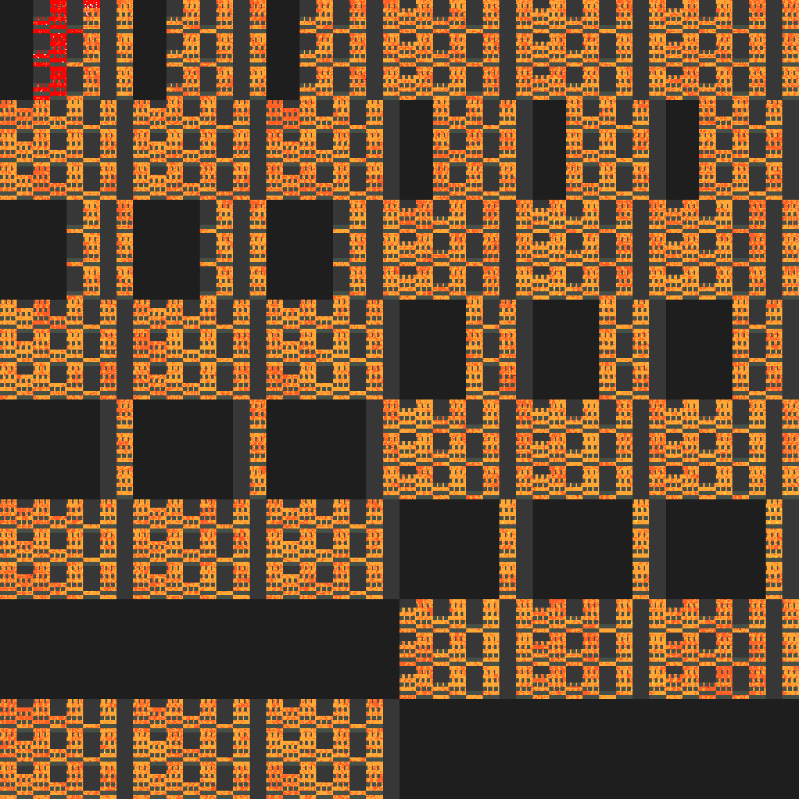
The above visualization is a sort of cross section of the search tree. The colour of each pixel corresponds to the depth reached from a particular node. If a node was never reached, the depth of the closest parent is used. The diagram is organized such that nodes closer in the search tree have corresponding pixels closer in the image.
In particular, each 2x2 square of pixels corresponds to a unique sequence of 4 moves that reaches that search node. The colour of each pixel determines the depth reached. For each 2x2 square, the minimum, lower quartile, middle quartile, and maximum of depths of the children are coloured.
You may have guessed that large holes are generated from our pruned_moves function, and you are indeed correct. Here is depth map for similar problem, but without move pruning.
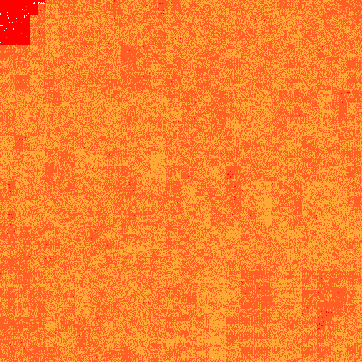
The way the nodes are mapped to the image, the search starts in to the top left working its way down until the first half is finished and then it works on the right half, eventually failing, increasing the depth limit and repeating until a solution is found. The top left should contain points at least as hot as rest since once the first solution is found it returns.
The depth map will allow us the evaluate the quality of heuristics. Ideally the majority of pixels in the depth map should be shades of grey and green, indicating a low search depth was needed before discarding the nodes.
More Heuristics
Before we create more heuristics, let's abstract to the core structure of them.
All of our heuristics will follow this same pattern.
- You have a number of buckets indexed from 0 to n.
- You have an index function which maps each state to one of the buckets.
- Then you assign single heuristic value for each bucket given by the number of moves required to solve the state with smallest solution in the bucket.
This is exactly what we did with our first heuristic, had 17 buckets labeled from 0 to 16, our index function was number solved tiles.
For consistency, we will use 64k buckets for each of our heuristics going forward. Since each bucket value is only 1 byte, our heuristic tables will only be 64kb, which easily fit into L2 cache. Also, making the bucket count 2^16 makes it easy to safely elide bound checks on the table lookup via a u16 cast.
For the most part, we are going to find our heuristics by trial and error. However, making full use of a heuristic requires you to find the smallest solution for a state in each bucket. When generating our first heuristic we search to a mere depth of 7. Searching much deeper drastically increases the time to generate the heuristics table.
I programmed a generic optimized heuristics table generator that we are going to use. In the generator the MoveSet is generic which we will utilize later. However, we still need to devise a MoveSet. Here is the trait.
pub trait MoveSet {
    fn all() -> &'static [Move];
    fn after(last_move:Move) -> &'static [Move];
}
And here is our current MoveSet.
struct AllMoves{};
impl MoveSet for AllMoves {
    fn all() -> &'static [Move] {
        use Move::*;
        &[R1x1, R1x2, R1x3,
          R2x1, R2x2, R2x3,
          R3x1, R3x2, R3x3,
          R4x1, R4x2, R4x3,
          C1x1, C1x2, C1x3,
          C2x1, C2x2, C2x3,
          C3x1, C3x2, C3x3,
          C4x1, C4x2, C4x3]
    }
    fn after(last_move:Move) -> &'static [Move] {
        pruned_moves(last_move)
    }
}
I'll explain how the generator's interface works via an example, generating our next heuristic.
generate_htable!(OptimalRowHeuristic {
    const MAX_DEPTH: u8 = 7;
    type MoveSet = AllMoves;
    fn index(state: TileMap) -> u16 {
        (state.raw() ^ TileMap::default().raw()) as u16
    }
});
The above macro generates code which once executed will output,
Generating HTable: OptimalRowHeuristic [max_depth:7, move_set_size:24, threads:2]
  Indices Reached: 43680 (66.7%)
  Mean Reached:    5.150065245759025
  Mean:            6.1005859375
Generation finished in 515.245604ms
Writing htable to: htables/OptimalRowHeuristic.table
Our second heuristic's index is just truncation of our state to the first 16 bits. If you recall our implementation, this corresponds to the packed tile positions in the first row. Two states belong to the same bucket if and only if the row of each state is the same.
You may notice that in the index we xor with the solved state — this converts our tile positions to bit-wise deltas. This is a normalization trick we will use later to exploit the symmetry of the puzzle. For now you can ignore it; xor-ing by a constant is information preserving.
Now let's look at the output,
Indices Reached: 43680 (66.7%): After searching to amax_depthof 7 only 43680 of the buckets contained any states. However, this is all possible states remember we're indexing on the 4 tile labels in the first row. Tiles labels cannot repeat, so there is exactly16*15*14*13 = 43680possible indices meaning we reached all buckets. It may seem wasteful that a third of the table is unused, however the computation required to meaningfully compress indices is much more expensive than the wasted space.Mean Reached: 5.15..: Out of all the buckets reached, the mean heuristic is 5.15.Mean: 6.10..: Out of all the buckets in the table the mean is 6.10. Note that in this case all possible states were reached this value is useless as none of the unreached values will ever be used. This value is high because we perform a complete search up to the maximum depth so we can safely assert that any bucket without state will need at least max_depth+1 moves to reach.
Note that these mean statistics are not the best way to judge the heuristic because they tell you only about the buckets and not directly about the heuristic of the actual states. Generally, higher mean is better, however since this value does not take into account the number of states inside each bucket, the mean heuristic for a given random state may differ significantly.
Enough talk, let's combine our new heuristic with our old one
fn hstat_solved(state: TileMap) -> u8 {
    let table = &[4, 6, 5, 4, 3, 4, 3, 5, 2, 2, 5, 4, 1, 4, 7, 7];
    if let Some(h) = table.get(state.tiles_solved() as usize) {*h} else {0}
}
fn hstat_row(state: TileMap) -> u8 {
    const TABLE: &[u8;65536] = include_bytes!(
        "../htables/OptimalBarHeuristic.table"
    );
    let index = (state.raw() ^ TileMap::default().raw()) as u16;
    TABLE[index as usize]
}

fn hstat(state: TileMap) -> u8 {
    std::cmp::max(
        hstat_row(state),
        hstat_solved(state),
    )
}
To combine our heuristic we just take the maximum. Since both are minimum bound the largest one is still a minimum bound.
Let's look at the benchmark.
Moves         Avg      Median         Min         Max  Solution
    3      1.29µs      1.20µs     64.00ns      5.33µs  [(0,3),2.7]
    4      1.62µs      1.27µs     39.00ns      7.83µs  [(0,4),3.3]
    5      4.57µs      3.13µs     37.00ns     43.06µs  [(0,5),4.2]
    6     31.41µs      5.74µs    322.00ns    450.61µs  [(1,6),4.8]
    7    113.34µs     17.99µs    415.00ns      1.93ms  [(2,7),5.6]
    8    752.13µs     56.43µs    346.00ns     14.57ms  [(2,8),6.4]
    9      8.54ms    321.88µs      1.88µs    159.55ms  [(4,9),7.3]
   10     44.61ms      1.75ms      1.49µs    541.07ms  [(4,10),8.0]
  *11    244.56ms      7.54ms      6.85µs       5.68s  [(5,11),8.4]
A sizable improvement: at depth 10 the average time dropped by 75%. The depth map improved as well but the difference is subtle; we will compare them soon.
Since our new table is based on the delta in the first row, it is actually row agnostic we can safely apply it any row. We can utilize this symmetry, easily with new implementation of hstat_row,
fn hstat_row(state: TileMap) -> u8 {
    const TABLE: &[u8;65536] = include_bytes!(
        "../htables/OptimalBarHeuristic.table"
    );
    let delta = (state.raw() ^ TileMap::default().raw()) as usize;
    max(max(TABLE[delta         & 0xffff], TABLE[(delta>>16) & 0xffff]),
        max(TABLE[(delta >> 32) & 0xffff], TABLE[(delta>>48) & 0xffff]))
}
Let's check out the benchmark
Moves         Avg      Median         Min         Max  Solution
    3      2.00µs      1.27µs     49.00ns     19.24µs  [(0,3),2.7]
    4      2.24µs      1.43µs     69.00ns     18.97µs  [(0,4),3.3]
    5      3.85µs      2.26µs     48.00ns     26.78µs  [(0,5),4.2]
    6     11.69µs      3.02µs    206.00ns    258.04µs  [(1,6),4.8]
    7     35.50µs      7.05µs    435.00ns    378.92µs  [(2,7),5.6]
    8    292.02µs     39.15µs    362.00ns      4.46ms  [(2,8),6.4]
    9      2.87ms    189.59µs      1.78µs     42.75ms  [(4,9),7.3]
   10     16.18ms    489.19µs    992.00ns    212.14ms  [(4,10),8.0]
   11     83.16ms      3.14ms      3.22µs       1.97s  [(5,11),8.4]
  *12    392.00ms     14.79ms    725.00ns       9.42s  [(2,12),9.1]
But we are not done utilizing symmetry yet. Since column and row moves are symmetric, we can use the row heuristic for columns as well. To motivate the implementation, consider the puzzle as a physical board. You scramble the puzzle with some sequence of moves. Now what if before you started, you rotated the physical board 90 degrees, then scrambled with the same moves, then rotated back? While the puzzle is rotated your column and row moves swap, but either way you end up with a puzzle that has the same number of moves in its smallest solution.
In group theory, rotation * scramble * rotation.inverse() is called a conjugation. Conjugation preserves many properties of the group, including minimum solution length, provided that conjugation maps the set of moves to itself.
Thus we improve our heuristic further with the following,
impl TileMap {
    fn rotate(self) -> TileMap {
        let rot90: TileMap = ArrayTileMap::new([
            0,  4,  8, 12,
            1,  5,  9, 13,
            2,  6, 10, 14,
            3,  7, 11, 15
        ]).into();
        rot90 * self * rot90.inverse()
    }
}
fn hstat(state: TileMap) -> u8 {
    max(hstat_row(state),
     max(hstat_solved(state), hstat_row(state.rotate())))
}
With this, however, we do not see a time save. Not because the heuristic was not improved, it was, but because of how expensive our heuristic function has become.
Moves         Avg      Median         Min         Max  Solution
   10     32.66ms      1.10ms      5.21µs    439.01ms  [(4,10),8.0]
   11    177.19ms      7.48ms     16.53µs       4.86s  [(5,11),8.4]
   12    847.09ms     35.97ms      2.79µs      18.63s  [(2,12),9.1]
The main slowdown is from the expensive rotation operation; let's optimize it
impl TileMap {
    #[inline]
    pub fn rotate(self) -> TileMap {
        let swap_mask = 0x3333_3333_3333_3333u64;
        let x = ((self.raw & swap_mask) << 2) | ((self.raw >> 2) & swap_mask);
        TileMap{raw:
         ((x & 0x000F_0000_0000_0000) >> 36) |
         ((x & 0x00F0_000F_0000_0000) >> 24) |
         ((x & 0x0F00_00F0_000F_0000) >> 12) |
         ( x & 0xF000_0F00_00F0_000F)        |
         ((x & 0x0000_F000_0F00_00F0) << 12) |
         ((x & 0x0000_0000_F000_0F00) << 24) |
         ((x & 0x0000_0000_0000_F000) << 36)
        }
    }
}
Now let's look at the benchmarks.
Moves         Avg      Median         Min         Max  Solution
    3      1.34µs      1.39µs     75.00ns      3.12µs  [(0,3),2.7]
    4      1.50µs      1.51µs     47.00ns      4.25µs  [(0,4),3.3]
    5      2.90µs      2.35µs     42.00ns     14.17µs  [(0,5),4.2]
    6      7.06µs      2.87µs    277.00ns     78.20µs  [(1,6),4.8]
    7     23.74µs      5.19µs    601.00ns    142.48µs  [(2,7),5.6]
    8    150.65µs     26.19µs    465.00ns      2.74ms  [(2,8),6.4]
    9      1.62ms    101.08µs      1.39µs     17.89ms  [(4,9),7.3]
   10      8.93ms    312.60µs      1.44µs    121.88ms  [(4,10),8.0]
   11     47.38ms      1.95ms      4.50µs       1.30s  [(5,11),8.4]
   12    223.56ms      9.44ms    902.00ns       4.95s  [(2,12),9.1]
Now we see some improvements, but notice the lower move count benchmarks actually regress as they benefit less from the improved heuristics but still pay the cost of increased computation to compute them.
Below is depth maps for the same input state, using the various heuristics we have tried.
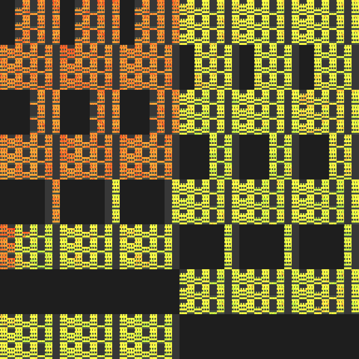
solved tiles
Improving the first heuristic
Our first heuristic was quite good given that it only had a bucket count of 17. Let's increase it. The basis for our first heuristic was number of solved tiles but we can improve by also storing which tiles are solved. Luckily, there are 16 bits in our index 1 bit for each of 16 tiles. Generating it is easy with a little bit of bit twiddling.
generate_htable!(OptimalSolvedHeuristic {
    const MAX_DEPTH: u8 = 8;
    type MoveSet = Phase1Moves;
    fn index(state: TileMap) -> u16 {
        let v = !(state.raw() ^ TileMap::default().raw());
        let v = (v >> 2) & v;
        let v = (v >> 1) & v & 0x1111_1111_1111_1111;
        (v | (v >> 15) | (v >> 30) | (v >> 45)) as u16
    }
});
Which outputs,
Generating HTable: OptimalSolvedHeuristic [max_depth:8, move_set_size:24, threads:2]
  Indices Reached: 64872 (99.0%)
  Mean Reached:    6.721317034821883
  Mean:            6.7445068359375
Generation finished in 12.009514206s
Writing htable to: htables/OptimalSolvedHeuristic.table
Nice, this heuristic is utilizing the table well at 99% usage and has quite a high mean of 6.7, higher than the row heuristic. Notice that it took 12s to generate the table — I am on my old dual-core Thinkpad laptop; on a faster computer this table builds easily in under a second. Anyway, we only have to build this table once.
Integrating our new heuristic is easy,
fn hstat_solved(state: TileMap) -> u8 {
    const TABLE: &[u8;65536] = include_bytes!(
        "../htables/OptimalSolvedHeuristic.table"
    );
    let v = !(state.raw() ^ TileMap::default().raw());
    let v = (v >> 2) & v;
    let v = (v >> 1) & v & 0x1111_1111_1111_1111;
    let index = (v | (v >> 15) | (v >> 30) | (v >> 45)) as u16;
    TABLE[index as usize]
}
Using our new heuristic we see a good improvement in performance.
Moves         Avg      Median         Min         Max  Solution
    3      1.61µs      1.29µs     62.00ns     19.98µs  [(0,3),2.7]
    4      1.73µs      1.38µs     40.00ns     19.09µs  [(0,4),3.3]
    5      2.32µs      1.76µs     31.00ns     15.83µs  [(0,5),4.2]
    6      3.93µs      2.35µs    287.00ns     25.60µs  [(1,6),4.8]
    7     10.49µs      3.50µs    594.00ns     66.12µs  [(2,7),5.6]
    8     71.74µs     10.01µs    438.00ns      1.15ms  [(2,8),6.4]
    9    770.64µs     56.13µs      1.47µs      8.42ms  [(4,9),7.3]
   10      5.56ms    179.30µs      1.54µs     68.69ms  [(4,10),8.0]
   11     29.46ms      1.03ms      2.41µs    822.39ms  [(5,11),8.4]
   12    141.62ms      4.96ms    722.00ns       2.97s  [(2,12),9.1]
  *13    230.04ms      2.69ms      1.98µs       3.31s  [(5,12),9.2]
 *100       3.09s       2.17s     14.11ms      23.39s  [(10,13),11.7]
 *100       2.47s       1.46s      3.77ms      15.76s  [(9,13),11.6]
We could continue adding more heuristics and performing more small optimizations. I have indeed done so and did see further performance improvements, reducing the solve time by about half.
What's Next: 2 Phase Solving
Our optimal solver works well but its runtime is still exponential in solution length. For fully scrambled inputs it averages around 3 seconds per solve. Optimality is a great property, but if you don't need it, there is a lot of performance left on the table.
The key idea of a 2 phase solver is splitting the problem into two simpler sub-problems, each with a shorter search depth. If both phases require an 8-move solution, the end result is a 16-move solution but each phase only took milliseconds instead of seconds. The tradeoff is solution quality, though you can mitigate this by generating multiple solutions and picking the shortest. This is exactly the approach used by the Cubie library's Rubik's cube solver and is how min2phase style solvers work in general.
For the tile puzzle, phase 1 might solve each row to contain only tiles of its colour (the easier sub-problem from the beginning of this post), and phase 2 would then sort within each row. Each phase has its own move set and heuristic tables, and the same IDA* machinery drives both.
The same core techniques carry over directly to the 3x3 Rubik's cube in the Cubie library. Starting from the tile puzzle we went from a naive O(24^n) brute-force search to an optimized solver that handles 12-move problems in milliseconds. Cubie applies these ideas (and a few more) to solve a fully scrambled Rubik's cube in under 10ms.